Feel free to click on the source to see how the code works or you can also simply scroll through to see the plots if you are in a rush!!!
Let’s start by importing our libraries!
Source
import matplotlib.pyplot as plt
import numpy as np
import pandas as pd
import seaborn as sns
Now we load the tsv data for our saliency peak data. We’ll also add an episode column!
Source
#read data set as pd
df= pd.read_csv("../output/Peak_scenes_merged.tsv", sep='\t')

#add episode column
df["episode_short"] = df["episode"].str.extract(r'(s\d+e\d+)', expand=False).str.upper()
We are now ready to plot some figures!
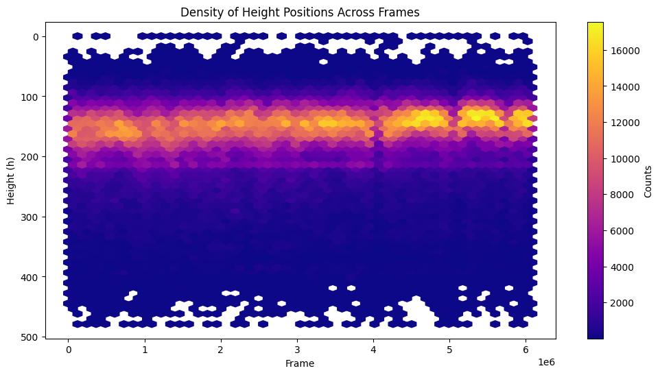
HEIGHT POSITION DENSITY (pixel space)
As you can see, the deepgaze ai shows us that the height position of the most salient point on screen stays relatively stable during seasons 1-6
Source
# plot for Density of Height Positions Across Frames
plt.figure(figsize=(12, 6))
plt.hexbin(df["frame"], df["h"], gridsize=50, cmap="plasma", mincnt=1)
plt.gca().invert_yaxis()
plt.colorbar(label="Counts")
plt.xlabel("Frame")
plt.ylabel("Height (h)")
plt.title("Density of Height Positions Across Frames")
plt.show()
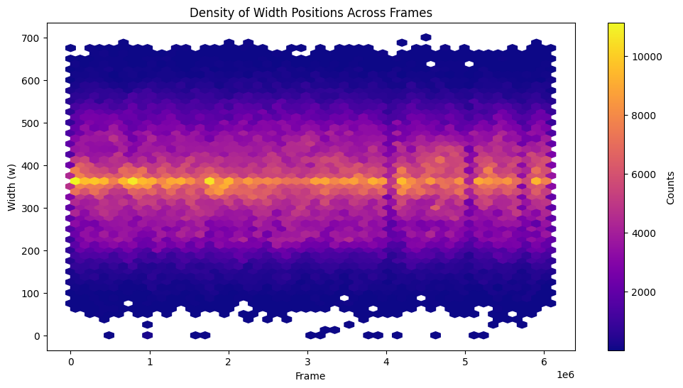
WIDTH POSITION DENSITY (pixel space)
Same goes for the width, the deepgaze ai shows us that the height position of the most salient point on screen stays relatively stable during seasons 1-6
Source
# plot for Density of width Positions Across Frames
plt.figure(figsize=(12, 6))
plt.hexbin(df["frame"], df["w"], gridsize=50, cmap="plasma", mincnt=1)
plt.colorbar(label="Counts")
plt.xlabel("Frame")
plt.ylabel("Width (w)")
plt.title("Density of Width Positions Across Frames")
plt.show()
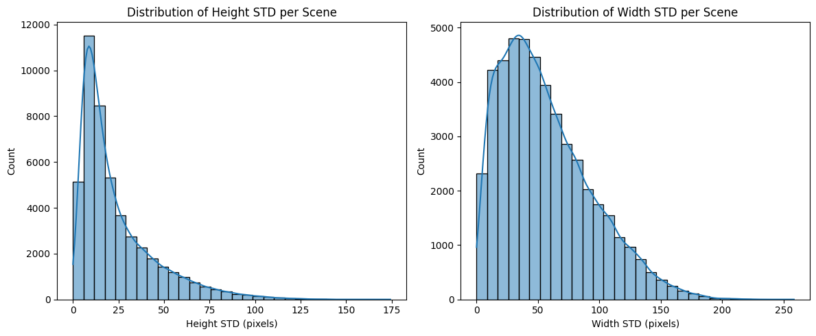
HEIGHT AND WIDTH DISTRIBUTION (pixel space)
For this next plot, we will nead some measures of central tendency like the mean and the standard deviation of the height and the width
With these plots, we see that the width and height values don’t vary that much
Source
# get stats on h and w depending on the scene_number
scene_stats = df.groupby(["episode_short", "global_scene_number"]).agg({
    "h": ["mean", "std", "min", "max"],
    "w": ["mean", "std", "min", "max"]
}).reset_index()

# Optional: flatten multi-level columns
scene_stats.columns = ["episode_short", "global_scene_number", "h_mean", "h_std", "h_min", "h_max",
                       "w_mean", "w_std", "w_min", "w_max"]
Source
#plot to show distribution of how much coordinates in scenes vary
plt.figure(figsize=(12,5))

plt.subplot(1,2,1)
sns.histplot(scene_stats["h_std"], bins=30, kde=True)
plt.title("Distribution of Height STD per Scene")
plt.xlabel("Height STD (pixels)")

plt.subplot(1,2,2)
sns.histplot(scene_stats["w_std"], bins=30, kde=True)
plt.title("Distribution of Width STD per Scene")
plt.xlabel("Width STD (pixels)")

plt.tight_layout()
plt.show()
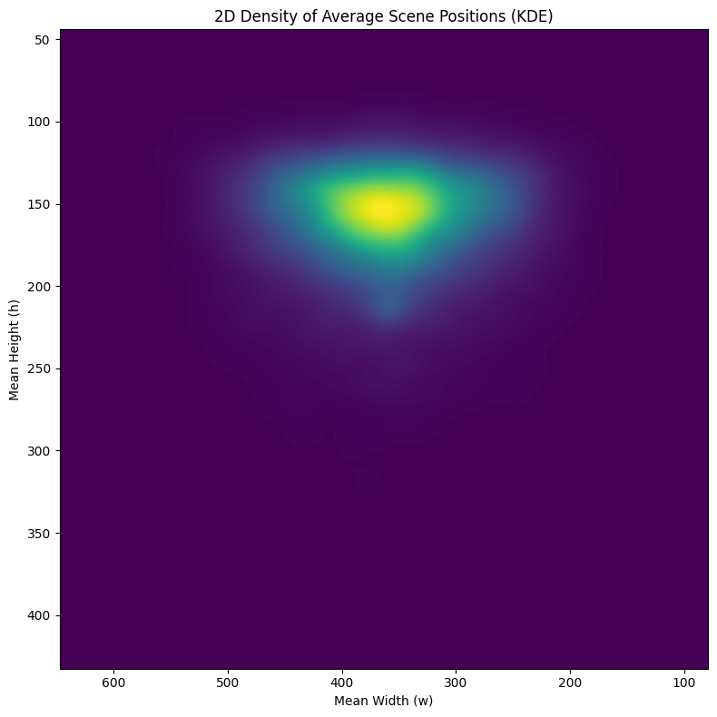
GAZE DENSITY IN PIXEL SPACE
Our final plot gives us a good idea of the area of saliency on the screen across the seasons. We see that it is concentrated in the upper third of the screen
Source
plt.figure(figsize=(8, 8))
sns.kdeplot(
    x=scene_stats["w_mean"],
    y=scene_stats["h_mean"],
    fill=True,  # fill the contours
    cmap="viridis",
    thresh=0,   # show full density (no threshold)
    levels=100  # number of contour levels (smoothness/detail)
)

plt.gca().invert_yaxis()
plt.gca().invert_xaxis()
plt.title("2D Density of Average Scene Positions (KDE)")
plt.xlabel("Mean Width (w)")
plt.ylabel("Mean Height (h)")
plt.tight_layout()
plt.show()